Panel Fixed Effects (PyMC)#
Panel data lets us follow the same units over time. Fixed effects regression controls for time-invariant unit heterogeneity by estimating unit-specific intercepts (dummy variables) or by using the within transformation (demeaning).
We introduce PanelRegression, compare dummy-variable and within estimators, and
connect the approach to Difference-in-Differences ({doc}notebooks/did_pymc).
Key ideas:
unit fixed effects remove time-invariant confounding
within transformation avoids large dummy matrices
two-way fixed effects add time indicators for common shocks
Note
This notebook uses small sampling settings for quick execution.
import arviz as az
import matplotlib.pyplot as plt
import numpy as np
import pandas as pd
from sklearn.linear_model import LinearRegression

import causalpy as cp
Outline#
Intuition and within transformation
Simulated example (ground truth)
Small panel with unit effects (dummy FE)
Large panel with within transformation
Two-way fixed effects and diagnostics
Exercises
Intuition: fixed effects and demeaning#
A standard unit fixed effects model is:
\(y_{it} = \alpha_i + \lambda_t + \beta D_{it} + X_{it}\gamma + \varepsilon_{it}\)
\(\alpha_i\) captures time-invariant unit characteristics
\(\lambda_t\) captures time shocks common to all units
\(D_{it}\) is a treatment indicator
The within transformation subtracts unit means:
\(\tilde{y}_{it} = y_{it} - \bar{y}_i\), and similarly for \(D_{it}\) and \(X_{it}\).
This removes \(\alpha_i\) and lets us estimate \(\beta\) without creating dummy variables. For two-way fixed effects, we also demean by time.
For a deeper econometric treatment, see Cunningham [2021].
Simulated panel data#
We simulate a balanced panel with unit effects, time effects, and a treatment effect. The goal is to recover the treatment effect while accounting for unit heterogeneity.
rng = np.random.default_rng(42)

n_units = 30
n_periods = 8
units = np.repeat(np.arange(n_units), n_periods)
times = np.tile(np.arange(n_periods), n_units)

unit_effects = rng.normal(0, 1.0, n_units)
time_effects = rng.normal(0, 0.5, n_periods)

x = rng.normal(0, 1.0, n_units * n_periods)
treatment = rng.binomial(1, 0.4, n_units * n_periods)
true_effect = 1.5

noise = rng.normal(0, 0.5, n_units * n_periods)

y = (
    unit_effects[units]
    + time_effects[times]
    + true_effect * treatment
    + 0.5 * x
    + noise
)

panel_df = pd.DataFrame(
    {
        "unit": units,
        "time": times,
        "x": x,
        "treatment": treatment,
        "y": y,
    }
)

panel_df.head()
| unit | time | x | treatment | y | |
|---|---|---|---|---|---|
| 0 | 0 | 0 | -0.824481 | 1 | 2.695840 |
| 1 | 0 | 1 | 0.650593 | 0 | -0.353673 |
| 2 | 0 | 2 | 0.743254 | 1 | 1.771561 |
| 3 | 0 | 3 | 0.543154 | 0 | 0.219147 |
| 4 | 0 | 4 | -0.665510 | 1 | 1.736902 |
def summarize_treatment(result, term="treatment", hdi_prob=0.9):
    labels = result.labels
    if term not in labels:
        raise ValueError(f"{term} not found in model labels")
    coef_index = labels.index(term)
    if isinstance(result.model, cp.pymc_models.PyMCModel):
        coeffs = az.extract(result.model.idata.posterior, var_names="beta")
        coeffs = coeffs.sel(treated_units=coeffs.coords["treated_units"].values[0])
        term_draws = coeffs.sel(coeffs=term)
        hdi = az.hdi(term_draws, hdi_prob=hdi_prob)
        return {
            "mean": float(term_draws.mean("sample")),
            "hdi_low": float(hdi.sel(hdi="lower")),
            "hdi_high": float(hdi.sel(hdi="higher")),
        }
    return {"mean": float(result.model.get_coeffs()[coef_index])}
Dummy-variable fixed effects#
Include unit and time indicators directly in the formula. This is straightforward and lets us inspect unit-specific coefficients.
dummies_model = cp.pymc_models.LinearRegression(
    sample_kwargs={
        "chains": 2,
        "draws": 200,
        "tune": 200,
        "target_accept": 0.9,
        "progressbar": False,
        "random_seed": 42,
    }
)

result_dummies = cp.PanelRegression(
    data=panel_df,
    formula="y ~ C(unit) + C(time) + treatment + x",
    unit_fe_variable="unit",
    time_fe_variable="time",
    fe_method="dummies",
    model=dummies_model,
)
Initializing NUTS using jitter+adapt_diag...
Multiprocess sampling (2 chains in 2 jobs)
NUTS: [beta, y_hat_sigma]
Sampling 2 chains for 200 tune and 200 draw iterations (400 + 400 draws total) took 0 seconds.
We recommend running at least 4 chains for robust computation of convergence diagnostics
The rhat statistic is larger than 1.01 for some parameters. This indicates problems during sampling. See https://arxiv.org/abs/1903.08008 for details
The effective sample size per chain is smaller than 100 for some parameters.  A higher number is needed for reliable rhat and ess computation. See https://arxiv.org/abs/1903.08008 for details
Sampling: [beta, y_hat, y_hat_sigma]
Sampling: [y_hat]
Sampling: [y_hat]
Sampling: [y_hat]
result_dummies.summary()
================================Panel Regression================================
Formula: y ~ C(unit) + C(time) + treatment + x
Units: 30 (unit)
Periods: 8 (time)
FE method: dummies
Model coefficients:
    Intercept      1.3, 94% HDI [0.98, 1.8]
    C(unit)[T.1]   -1.2, 94% HDI [-1.7, -0.77]
    C(unit)[T.2]   0.5, 94% HDI [-0.018, 1]
    C(unit)[T.3]   0.35, 94% HDI [-0.12, 0.77]
    C(unit)[T.4]   -2.4, 94% HDI [-2.9, -1.9]
    C(unit)[T.5]   -1.5, 94% HDI [-2, -1]
    C(unit)[T.6]   -0.37, 94% HDI [-0.8, 0.042]
    C(unit)[T.7]   -0.69, 94% HDI [-1.2, -0.27]
    C(unit)[T.8]   -0.46, 94% HDI [-0.93, -0.0019]
    C(unit)[T.9]   -1.3, 94% HDI [-1.7, -0.77]
    C(unit)[T.10]  0.5, 94% HDI [0.077, 0.92]
    C(unit)[T.11]  0.39, 94% HDI [-0.062, 0.82]
    C(unit)[T.12]  -0.34, 94% HDI [-0.77, 0.083]
    C(unit)[T.13]  0.79, 94% HDI [0.31, 1.2]
    C(unit)[T.14]  0.11, 94% HDI [-0.38, 0.57]
    C(unit)[T.15]  -1.3, 94% HDI [-1.8, -0.8]
    C(unit)[T.16]  0.12, 94% HDI [-0.36, 0.58]
    C(unit)[T.17]  -1.2, 94% HDI [-1.6, -0.71]
    C(unit)[T.18]  0.47, 94% HDI [-0.049, 0.93]
    C(unit)[T.19]  -0.68, 94% HDI [-1.1, -0.19]
    C(unit)[T.20]  -0.51, 94% HDI [-0.98, -0.054]
    C(unit)[T.21]  -0.88, 94% HDI [-1.4, -0.42]
    C(unit)[T.22]  1, 94% HDI [0.49, 1.6]
    C(unit)[T.23]  -0.9, 94% HDI [-1.4, -0.39]
    C(unit)[T.24]  -0.87, 94% HDI [-1.4, -0.39]
    C(unit)[T.25]  -0.86, 94% HDI [-1.3, -0.43]
    C(unit)[T.26]  -0.052, 94% HDI [-0.61, 0.4]
    C(unit)[T.27]  0.14, 94% HDI [-0.34, 0.62]
    C(unit)[T.28]  0.044, 94% HDI [-0.46, 0.59]
    C(unit)[T.29]  0.2, 94% HDI [-0.24, 0.65]
    C(time)[T.1]   -1.2, 94% HDI [-1.5, -0.93]
    C(time)[T.2]   -1.3, 94% HDI [-1.5, -1.1]
    C(time)[T.3]   -1.4, 94% HDI [-1.7, -1.2]
    C(time)[T.4]   -0.66, 94% HDI [-0.89, -0.41]
    C(time)[T.5]   -0.47, 94% HDI [-0.76, -0.23]
    C(time)[T.6]   -1.2, 94% HDI [-1.4, -0.9]
    C(time)[T.7]   -1.5, 94% HDI [-1.7, -1.2]
    treatment      1.5, 94% HDI [1.4, 1.7]
    x              0.46, 94% HDI [0.4, 0.53]
    y_hat_sigma    0.53, 94% HDI [0.48, 0.58]
Within transformation#
The within estimator demeans the data by unit (and time, if provided), which avoids creating large dummy matrices. This is preferred for large panels.
within_model = cp.pymc_models.LinearRegression(
    sample_kwargs={
        "chains": 2,
        "draws": 200,
        "tune": 200,
        "target_accept": 0.9,
        "progressbar": False,
        "random_seed": 42,
    }
)

result_within = cp.PanelRegression(
    data=panel_df,
    formula="y ~ treatment + x",
    unit_fe_variable="unit",
    time_fe_variable="time",
    fe_method="within",
    model=within_model,
)
/Users/benjamv/git/CausalPy/causalpy/experiments/panel_regression.py:146: FutureWarning: Setting an item of incompatible dtype is deprecated and will raise in a future error of pandas. Value '[ 0.25  -0.75   0.25  -0.75   0.25   0.25   0.25   0.25   0.5    0.5
  0.5   -0.5   -0.5   -0.5    0.5   -0.5   -0.125  0.875 -0.125 -0.125
 -0.125 -0.125 -0.125 -0.125 -0.375 -0.375 -0.375  0.625 -0.375  0.625
  0.625 -0.375 -0.5   -0.5    0.5    0.5    0.5   -0.5    0.5   -0.5
  0.375 -0.625  0.375  0.375 -0.625  0.375 -0.625  0.375 -0.625  0.375
 -0.625  0.375  0.375 -0.625  0.375  0.375  0.75  -0.25  -0.25  -0.25
  0.75  -0.25  -0.25  -0.25  -0.375 -0.375  0.625  0.625 -0.375 -0.375
  0.625 -0.375 -0.5   -0.5    0.5   -0.5    0.5    0.5   -0.5    0.5
  0.75  -0.25  -0.25  -0.25  -0.25  -0.25   0.75  -0.25  -0.5    0.5
 -0.5    0.5    0.5   -0.5   -0.5    0.5    0.375  0.375 -0.625  0.375
  0.375 -0.625 -0.625  0.375 -0.25  -0.25   0.75  -0.25  -0.25  -0.25
 -0.25   0.75   0.375 -0.625  0.375  0.375 -0.625  0.375 -0.625  0.375
  0.5    0.5   -0.5    0.5   -0.5   -0.5   -0.5    0.5   -0.5    0.5
  0.5   -0.5   -0.5   -0.5    0.5    0.5   -0.75   0.25  -0.75   0.25
  0.25   0.25   0.25   0.25  -0.375 -0.375 -0.375 -0.375  0.625  0.625
  0.625 -0.375  0.375 -0.625 -0.625  0.375  0.375  0.375 -0.625  0.375
 -0.375  0.625  0.625 -0.375 -0.375 -0.375  0.625 -0.375  0.5    0.5
 -0.5   -0.5    0.5   -0.5   -0.5    0.5    0.75   0.75  -0.25  -0.25
 -0.25  -0.25  -0.25  -0.25  -0.25  -0.25  -0.25   0.75   0.75  -0.25
 -0.25  -0.25   0.     0.     0.     0.     0.     0.     0.     0.
  0.375  0.375  0.375 -0.625  0.375 -0.625 -0.625  0.375 -0.5   -0.5
  0.5    0.5    0.5   -0.5   -0.5    0.5   -0.25   0.75  -0.25  -0.25
 -0.25   0.75  -0.25  -0.25  -0.375 -0.375 -0.375  0.625 -0.375  0.625
  0.625 -0.375 -0.5    0.5   -0.5   -0.5    0.5    0.5    0.5   -0.5  ]' has dtype incompatible with int64, please explicitly cast to a compatible dtype first.
  data.loc[:, numeric_cols] = data[numeric_cols].sub(group_means)
Initializing NUTS using jitter+adapt_diag...
Multiprocess sampling (2 chains in 2 jobs)
NUTS: [beta, y_hat_sigma]
Sampling 2 chains for 200 tune and 200 draw iterations (400 + 400 draws total) took 0 seconds.
We recommend running at least 4 chains for robust computation of convergence diagnostics
The rhat statistic is larger than 1.01 for some parameters. This indicates problems during sampling. See https://arxiv.org/abs/1903.08008 for details
Sampling: [beta, y_hat, y_hat_sigma]
Sampling: [y_hat]
Sampling: [y_hat]
Sampling: [y_hat]
result_within.summary()
================================Panel Regression================================
Formula: y ~ treatment + x
Units: 30 (unit)
Periods: 8 (time)
FE method: within
Model coefficients:
    Intercept    0.00086, 94% HDI [-0.051, 0.056]
    treatment    1.6, 94% HDI [1.4, 1.7]
    x            0.46, 94% HDI [0.39, 0.54]
    y_hat_sigma  0.49, 94% HDI [0.44, 0.53]
Compare treatment estimates#
Both approaches should recover the true treatment effect on this simulated panel.
summary_dummies = summarize_treatment(result_dummies)
summary_within = summarize_treatment(result_within)

pd.DataFrame(
    {
        "method": ["dummies", "within"],
        "estimate": [summary_dummies["mean"], summary_within["mean"]],
        "true_effect": [true_effect, true_effect],
    }
)
---------------------------------------------------------------------------
ValueError                                Traceback (most recent call last)
Cell In[9], line 1
----> 1 summary_dummies = summarize_treatment(result_dummies)
      2 summary_within = summarize_treatment(result_within)
      4 pd.DataFrame(
      5     {
      6         "method": ["dummies", "within"],
   (...)      9     }
     10 )

Cell In[3], line 10, in summarize_treatment(result, term, hdi_prob)
      8     coeffs = coeffs.sel(treated_units=coeffs.coords["treated_units"].values[0])
      9     term_draws = coeffs.sel(coeffs=term)
---> 10     hdi = az.hdi(term_draws, hdi_prob=hdi_prob)
     11     return {
     12         "mean": float(term_draws.mean("sample")),
     13         "hdi_low": float(hdi.sel(hdi="lower")),
     14         "hdi_high": float(hdi.sel(hdi="higher")),
     15     }
     16 return {"mean": float(result.model.get_coeffs()[coef_index])}

File ~/miniforge3/envs/CausalPy/lib/python3.14/site-packages/arviz/stats/stats.py:582, in hdi(ary, hdi_prob, circular, multimodal, skipna, group, var_names, filter_vars, coords, max_modes, dask_kwargs, **kwargs)
    579 ary = ary[var_names] if var_names else ary
    581 hdi_coord = xr.DataArray(["lower", "higher"], dims=["hdi"], attrs=dict(hdi_prob=hdi_prob))
--> 582 hdi_data = _wrap_xarray_ufunc(
    583     func, ary, func_kwargs=func_kwargs, dask_kwargs=dask_kwargs, **kwargs
    584 ).assign_coords({"hdi": hdi_coord})
    585 hdi_data = hdi_data.dropna("mode", how="all") if multimodal else hdi_data
    586 return hdi_data.x.values if isarray else hdi_data

File ~/miniforge3/envs/CausalPy/lib/python3.14/site-packages/arviz/utils.py:766, in conditional_dask.<locals>.wrapper(*args, **kwargs)
    763 @functools.wraps(func)
    764 def wrapper(*args, **kwargs):
    765     if not Dask.dask_flag:
--> 766         return func(*args, **kwargs)
    767     user_kwargs = kwargs.pop("dask_kwargs", None)
    768     if user_kwargs is None:

File ~/miniforge3/envs/CausalPy/lib/python3.14/site-packages/arviz/stats/stats_utils.py:240, in wrap_xarray_ufunc(ufunc, ufunc_kwargs, func_args, func_kwargs, dask_kwargs, *datasets, **kwargs)
    236 kwargs.setdefault("output_core_dims", tuple([] for _ in range(ufunc_kwargs.get("n_output", 1))))
    238 callable_ufunc = make_ufunc(ufunc, **ufunc_kwargs)
--> 240 return apply_ufunc(
    241     callable_ufunc, *datasets, *func_args, kwargs=func_kwargs, **dask_kwargs, **kwargs
    242 )

File ~/miniforge3/envs/CausalPy/lib/python3.14/site-packages/xarray/computation/apply_ufunc.py:1254, in apply_ufunc(func, input_core_dims, output_core_dims, exclude_dims, vectorize, join, dataset_join, dataset_fill_value, keep_attrs, kwargs, dask, output_dtypes, output_sizes, meta, dask_gufunc_kwargs, on_missing_core_dim, *args)
   1252 # feed datasets apply_variable_ufunc through apply_dataset_vfunc
   1253 elif any(is_dict_like(a) for a in args):
-> 1254     return apply_dataset_vfunc(
   1255         variables_vfunc,
   1256         *args,
   1257         signature=signature,
   1258         join=join,
   1259         exclude_dims=exclude_dims,
   1260         dataset_join=dataset_join,
   1261         fill_value=dataset_fill_value,
   1262         keep_attrs=keep_attrs,
   1263         on_missing_core_dim=on_missing_core_dim,
   1264     )
   1265 # feed DataArray apply_variable_ufunc through apply_dataarray_vfunc
   1266 elif any(isinstance(a, DataArray) for a in args):

File ~/miniforge3/envs/CausalPy/lib/python3.14/site-packages/xarray/computation/apply_ufunc.py:525, in apply_dataset_vfunc(func, signature, join, dataset_join, fill_value, exclude_dims, keep_attrs, on_missing_core_dim, *args)
    520 list_of_coords, list_of_indexes = build_output_coords_and_indexes(
    521     args, signature, exclude_dims, combine_attrs=keep_attrs
    522 )
    523 args = tuple(getattr(arg, "data_vars", arg) for arg in args)
--> 525 result_vars = apply_dict_of_variables_vfunc(
    526     func,
    527     *args,
    528     signature=signature,
    529     join=dataset_join,
    530     fill_value=fill_value,
    531     on_missing_core_dim=on_missing_core_dim,
    532 )
    534 out: Dataset | tuple[Dataset, ...]
    535 if signature.num_outputs > 1:

File ~/miniforge3/envs/CausalPy/lib/python3.14/site-packages/xarray/computation/apply_ufunc.py:452, in apply_dict_of_variables_vfunc(func, signature, join, fill_value, on_missing_core_dim, *args)
    450     result_vars[name] = func(*variable_args)
    451 elif on_missing_core_dim == "raise":
--> 452     raise ValueError(core_dim_present)
    453 elif on_missing_core_dim == "copy":
    454     result_vars[name] = variable_args[0]

ValueError: Missing core dims {'draw', 'chain'} from arg number 1 on a variable named `beta`:
<xarray.Variable (sample: 400)> Size: 3kB
array([1.57057215, 1.57013218, 1.52397914, 1.67220542, 1.57199663,
       1.48858332, 1.62414239, 1.59612805, 1.61941031, 1.48311572,
       1.55409155, 1.46225304, 1.62853793, 1.57174023, 1.45981961,
       1.43797817, 1.5725262 , 1.41007586, 1.56005522, 1.53150886,
       1.59106391, 1.69238209, 1.39518096, 1.50074308, 1.48426758,
       1.43338129, 1.43542312, 1.52337746, 1.59527211, 1.49224427,
       1.51853794, 1.46921417, 1.42001541, 1.58278358, 1.56137972,
       1.46111782, 1.66690219, 1.48422342, 1.5322973 , 1.37511373,
       1.57748691, 1.60392727, 1.53395418, 1.54547357, 1.48840353,
       1.58540911, 1.53923651, 1.57491693, 1.59193645, 1.52111579,
       1.59377557, 1.62198151, 1.66375968, 1.46400664, 1.45485061,
       1.43789605, 1.45574952, 1.61556478, 1.59524657, 1.38420266,
       1.70899059, 1.42747921, 1.49855039, 1.38782131, 1.68140838,
       1.41037593, 1.48943489, 1.58421277, 1.49547401, 1.52629381,
       1.49427581, 1.48369737, 1.60442436, 1.59686808, 1.5381013 ,
       1.54890706, 1.54965856, 1.49708358, 1.62404463, 1.3780108 ,
       1.48835817, 1.57392344, 1.54192886, 1.41337148, 1.63429138,
       1.47031386, 1.65535277, 1.67847077, 1.65838085, 1.4156537 ,
       1.55772195, 1.63980256, 1.45861128, 1.4992685 , 1.60196989,
       1.42584673, 1.61286327, 1.47843439, 1.60812938, 1.47062599,
...
       1.76378304, 1.64922437, 1.63165842, 1.47822201, 1.53074654,
       1.52156593, 1.52512897, 1.5010676 , 1.54789963, 1.59020171,
       1.64428639, 1.61091733, 1.61284562, 1.66452212, 1.654388  ,
       1.53417463, 1.64731081, 1.52761996, 1.61387681, 1.52253089,
       1.48851225, 1.63399815, 1.6604335 , 1.46039995, 1.45842661,
       1.58134379, 1.55929596, 1.4343112 , 1.65302568, 1.59766103,
       1.42344278, 1.62788841, 1.38784288, 1.61464037, 1.42898617,
       1.64803652, 1.49073468, 1.52276313, 1.54301403, 1.6472306 ,
       1.52846837, 1.57455907, 1.53535044, 1.43081709, 1.40448809,
       1.58335175, 1.49761928, 1.55852081, 1.48032396, 1.60981521,
       1.50565241, 1.57240499, 1.59260127, 1.52788097, 1.53215695,
       1.64507772, 1.56609488, 1.55847735, 1.52242583, 1.53433524,
       1.48969664, 1.52673094, 1.50636654, 1.59744064, 1.62539462,
       1.64019703, 1.63113337, 1.49389279, 1.51469643, 1.52467834,
       1.5790893 , 1.53029313, 1.49987184, 1.62556222, 1.56224888,
       1.59643249, 1.45708277, 1.61014969, 1.45347358, 1.50218775,
       1.55363609, 1.58426462, 1.65154348, 1.45866231, 1.57601384,
       1.51058246, 1.52644452, 1.50569851, 1.63158278, 1.43491539,
       1.56778054, 1.59536179, 1.46522363, 1.60167736, 1.55641865,
       1.47188592, 1.56245121, 1.56644924, 1.53612121, 1.55229765])

Either add the core dimension, or if passing a dataset alternatively pass `on_missing_core_dim` as `copy` or `drop`.
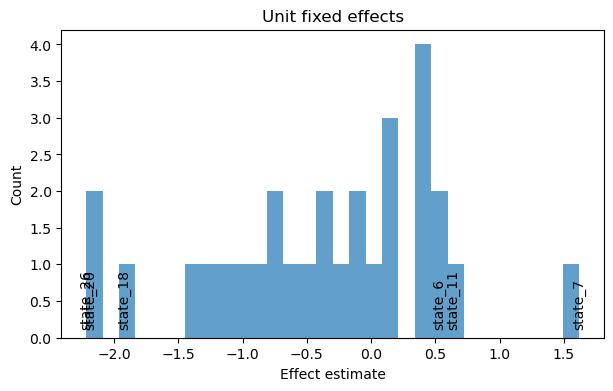
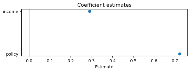
Example: small panel with unit effects (dummy FE)#
For smaller panels, dummy variables are practical and give unit-specific effects. Here we simulate a “states × years” panel and use an OLS model for speed.
rng = np.random.default_rng(7)
n_states = 30
n_years = 10
states = np.repeat([f"state_{i}" for i in range(n_states)], n_years)
years = np.tile(np.arange(2000, 2000 + n_years), n_states)
state_effects = rng.normal(0, 1.0, n_states)
year_effects = rng.normal(0, 0.3, n_years)
policy = rng.binomial(1, 0.4, n_states * n_years)
income = rng.normal(0, 1.0, n_states * n_years)
small_df = pd.DataFrame(
{
"state": states,
"year": years,
"policy": policy,
"income": income,
"y": (
state_effects[[int(s.split("_")[1]) for s in states]]
+ year_effects[years - 2000]
+ 0.8 * policy
+ 0.3 * income
+ rng.normal(0, 0.5, n_states * n_years)
),
}
)
small_result = cp.PanelRegression(
data=small_df,
formula="y ~ C(state) + C(year) + policy + income",
unit_fe_variable="state",
time_fe_variable="year",
fe_method="dummies",
model=LinearRegression(),
)
small_result.plot_coefficients(var_names=["policy", "income"])
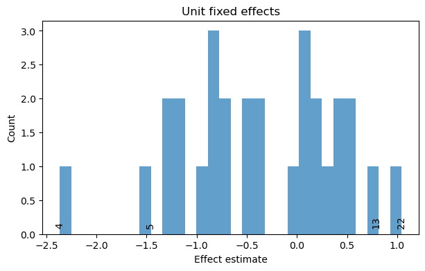
small_result.plot_unit_effects(label_extreme=3)
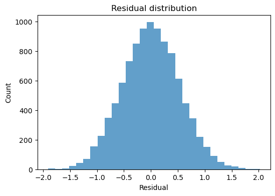
Example: large panel with within transformation#
For large panels, the within estimator avoids creating thousands of dummy columns. We use an OLS model here to keep computation fast.
rng = np.random.default_rng(21)

n_units_large = 2000
n_periods_large = 5
units_large = np.repeat(np.arange(n_units_large), n_periods_large)
times_large = np.tile(np.arange(n_periods_large), n_units_large)

unit_effects_large = rng.normal(0, 1.0, n_units_large)
time_effects_large = rng.normal(0, 0.2, n_periods_large)

x_large = rng.normal(0, 1.0, n_units_large * n_periods_large)
treatment_large = rng.binomial(1, 0.3, n_units_large * n_periods_large)

large_df = pd.DataFrame(
    {
        "id": units_large,
        "time": times_large,
        "x": x_large,
        "treatment": treatment_large,
        "y": (
            unit_effects_large[units_large]
            + time_effects_large[times_large]
            + 1.2 * treatment_large
            + 0.4 * x_large
            + rng.normal(0, 0.6, n_units_large * n_periods_large)
        ),
    }
)

large_result = cp.PanelRegression(
    data=large_df,
    formula="y ~ treatment + x",
    unit_fe_variable="id",
    time_fe_variable="time",
    fe_method="within",
    model=LinearRegression(),
)
/Users/benjamv/git/CausalPy/causalpy/experiments/panel_regression.py:146: FutureWarning: Setting an item of incompatible dtype is deprecated and will raise in a future error of pandas. Value '[-0.2  0.8 -0.2 ... -0.2 -0.2 -0.2]' has dtype incompatible with int64, please explicitly cast to a compatible dtype first.
  data.loc[:, numeric_cols] = data[numeric_cols].sub(group_means)
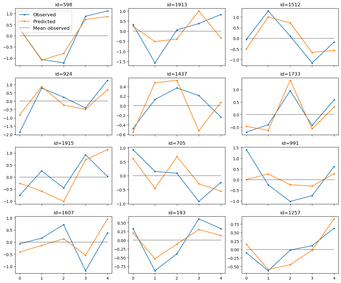
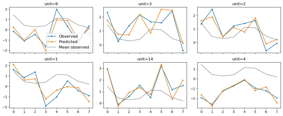
large_result.plot_trajectories(n_sample=12, select="random");
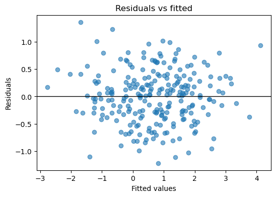
large_result.plot_residuals(kind="histogram");
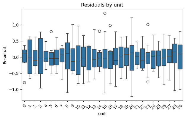
Diagnostics and visualization#
The plotting helpers focus on covariate coefficients, unit effects (for dummy models), trajectory subsets, and residual diagnostics. For large panels, the plotting methods sample units automatically.
Note
Within-transformed models plot demeaned outcomes and predictions.
result_dummies.plot_coefficients()
---------------------------------------------------------------------------
ValueError                                Traceback (most recent call last)
Cell In[16], line 1
----> 1 result_dummies.plot_coefficients()

File ~/git/CausalPy/causalpy/experiments/panel_regression.py:245, in PanelRegression.plot_coefficients(self, var_names, hdi_prob)
    243 coeffs = coeffs.sel(treated_units=coeffs.coords["treated_units"].values[0])
    244 coeffs = coeffs.sel(coeffs=var_names)
--> 245 hdi = az.hdi(coeffs, hdi_prob=hdi_prob)
    246 means = coeffs.mean("sample").values
    247 lower = hdi.sel(hdi="lower").values

File ~/miniforge3/envs/CausalPy/lib/python3.14/site-packages/arviz/stats/stats.py:582, in hdi(ary, hdi_prob, circular, multimodal, skipna, group, var_names, filter_vars, coords, max_modes, dask_kwargs, **kwargs)
    579 ary = ary[var_names] if var_names else ary
    581 hdi_coord = xr.DataArray(["lower", "higher"], dims=["hdi"], attrs=dict(hdi_prob=hdi_prob))
--> 582 hdi_data = _wrap_xarray_ufunc(
    583     func, ary, func_kwargs=func_kwargs, dask_kwargs=dask_kwargs, **kwargs
    584 ).assign_coords({"hdi": hdi_coord})
    585 hdi_data = hdi_data.dropna("mode", how="all") if multimodal else hdi_data
    586 return hdi_data.x.values if isarray else hdi_data

File ~/miniforge3/envs/CausalPy/lib/python3.14/site-packages/arviz/utils.py:766, in conditional_dask.<locals>.wrapper(*args, **kwargs)
    763 @functools.wraps(func)
    764 def wrapper(*args, **kwargs):
    765     if not Dask.dask_flag:
--> 766         return func(*args, **kwargs)
    767     user_kwargs = kwargs.pop("dask_kwargs", None)
    768     if user_kwargs is None:

File ~/miniforge3/envs/CausalPy/lib/python3.14/site-packages/arviz/stats/stats_utils.py:240, in wrap_xarray_ufunc(ufunc, ufunc_kwargs, func_args, func_kwargs, dask_kwargs, *datasets, **kwargs)
    236 kwargs.setdefault("output_core_dims", tuple([] for _ in range(ufunc_kwargs.get("n_output", 1))))
    238 callable_ufunc = make_ufunc(ufunc, **ufunc_kwargs)
--> 240 return apply_ufunc(
    241     callable_ufunc, *datasets, *func_args, kwargs=func_kwargs, **dask_kwargs, **kwargs
    242 )

File ~/miniforge3/envs/CausalPy/lib/python3.14/site-packages/xarray/computation/apply_ufunc.py:1254, in apply_ufunc(func, input_core_dims, output_core_dims, exclude_dims, vectorize, join, dataset_join, dataset_fill_value, keep_attrs, kwargs, dask, output_dtypes, output_sizes, meta, dask_gufunc_kwargs, on_missing_core_dim, *args)
   1252 # feed datasets apply_variable_ufunc through apply_dataset_vfunc
   1253 elif any(is_dict_like(a) for a in args):
-> 1254     return apply_dataset_vfunc(
   1255         variables_vfunc,
   1256         *args,
   1257         signature=signature,
   1258         join=join,
   1259         exclude_dims=exclude_dims,
   1260         dataset_join=dataset_join,
   1261         fill_value=dataset_fill_value,
   1262         keep_attrs=keep_attrs,
   1263         on_missing_core_dim=on_missing_core_dim,
   1264     )
   1265 # feed DataArray apply_variable_ufunc through apply_dataarray_vfunc
   1266 elif any(isinstance(a, DataArray) for a in args):

File ~/miniforge3/envs/CausalPy/lib/python3.14/site-packages/xarray/computation/apply_ufunc.py:525, in apply_dataset_vfunc(func, signature, join, dataset_join, fill_value, exclude_dims, keep_attrs, on_missing_core_dim, *args)
    520 list_of_coords, list_of_indexes = build_output_coords_and_indexes(
    521     args, signature, exclude_dims, combine_attrs=keep_attrs
    522 )
    523 args = tuple(getattr(arg, "data_vars", arg) for arg in args)
--> 525 result_vars = apply_dict_of_variables_vfunc(
    526     func,
    527     *args,
    528     signature=signature,
    529     join=dataset_join,
    530     fill_value=fill_value,
    531     on_missing_core_dim=on_missing_core_dim,
    532 )
    534 out: Dataset | tuple[Dataset, ...]
    535 if signature.num_outputs > 1:

File ~/miniforge3/envs/CausalPy/lib/python3.14/site-packages/xarray/computation/apply_ufunc.py:452, in apply_dict_of_variables_vfunc(func, signature, join, fill_value, on_missing_core_dim, *args)
    450     result_vars[name] = func(*variable_args)
    451 elif on_missing_core_dim == "raise":
--> 452     raise ValueError(core_dim_present)
    453 elif on_missing_core_dim == "copy":
    454     result_vars[name] = variable_args[0]

ValueError: Missing core dims {'draw', 'chain'} from arg number 1 on a variable named `beta`:
<xarray.Variable (coeffs: 3, sample: 400)> Size: 10kB
array([[1.0620972 , 1.07823805, 1.06763979, ..., 1.52455217, 1.59538179,
        1.63559953],
       [1.57057215, 1.57013218, 1.52397914, ..., 1.56644924, 1.53612121,
        1.55229765],
       [0.49783233, 0.47749703, 0.45853052, ..., 0.47983782, 0.45401651,
        0.49046701]], shape=(3, 400))

Either add the core dimension, or if passing a dataset alternatively pass `on_missing_core_dim` as `copy` or `drop`.
result_dummies.plot_unit_effects(label_extreme=2);
result_dummies.plot_trajectories(n_sample=6, select="random");
result_dummies.plot_residuals(kind="scatter");
result_dummies.plot_residuals(kind="qq");
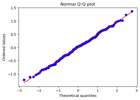
result_dummies.plot_residuals(by="unit");
Two-way fixed effects#
Setting time_fe_variable applies time fixed effects alongside unit effects. This is
closely related to two-way fixed effects models used in Difference-in-Differences
settings ({doc}notebooks/did_pymc) and relies on the parallel trends assumption.
For panel data foundations, see :footcite:p:cunningham2021causal.
Comparison to random effects#
Random effects models assume unit effects are uncorrelated with covariates. Fixed effects relax that assumption by conditioning on unit-specific intercepts, but do not estimate time-invariant covariates. In practice, FE is preferred when unit effects are likely correlated with treatment or controls.
Exercises#
Drop the time fixed effects and compare the treatment estimate.
Increase unit heterogeneity and compare dummy vs within estimates.
Use
plot_trajectories(select="extreme")and inspect the units selected.
References#
Scott Cunningham. Causal inference: The mixtape. Yale university press, 2021.